Classifying Flowers Part 1: Data

Everybody loves plants. So we'll continue our descent by building a neural network that can do something with plants. This construct will be able to take characteristics that describe a plant and, if we're good enough, hopefully the neural network will be able to tell us with accuracy what type of plant it is.

To do this, we'll use the Iris flowers dataset, which contains 150 samples of 3 different species (50 samples each). The species in this dataset are Iris setosa, Iris versicolor, and Iris virginica.

The dataset can be found at the following links.
Data: https://archive.ics.uci.edu/ml/machine-learning-databases/iris/iris.data
ReadME: https://archive.ics.uci.edu/ml/machine-learning-databases/iris/iris.names

Here's a screenshot of the data we'll be working with:

Initially, this data doesn't look too exciting and if it at all confuses you, you're perfectly normal. But we can figure some immediate information just from looking at the format of this data. Firstly, the data is given in rows of comma-delimited lists. There appears to be 4 decimal values followed by a single string value in each row. Thus there are 5 values in each row.

We can find even more information about the data by looking at the ReadME.

Bullet point 7 in the ReadME gives some information regarding what the different values in each row mean. The columns are:

1. sepal length (cm)
2. sepal width (cm)
3. petal length (cm)
4. petal width (cm)
5. species

So we can consider each row in the given data to be a specific plant, and for each plant, we are given some characteristics that describe it (i.e. sepal and petal measurements) as well as what type of plant it is (i.e. the species). 

Note: for those of you that don't know what a sepal is, here's an anatomically perfect depiction of the labelled parts of a flower: 

(stolen from https://extension.illinois.edu/gpe/images/flowerpartssepal.gif)

So cool, we have data with a bunch of instances of plants and we can try to throw deep learning at it to see if we can train a neural network to correctly classify them. I'm going to save the data at C:\Blog\iris.data.csv (the link tries to coerce you to saving the data as iris.data.txt so be sure to change the file's extension to .csv) and we'll try to do everything in R, which we installed in Blog Post 2. 

We'll open up RStudio and in the console, use the following commands to read the data into a dataframe, which is like a table in R that we can manipulate:

Please note that if you don't understand what all this R code means, that's okay. I'll be including comments to detail every action that's taken so people that are either learning R or don't really care to dip their hands in the statisticians' swimming pool can follow along. 

After loading the data into an R DataFrame, we'll have to partition it into training and test sets. So it's probably a good time to develop an understanding of training and test sets. 

When you want to train any predictive model (thing that makes predictions), you'll first throw examples at it and somehow it learns. We won't go into the details of how learning occurs because it's too math-y for this blog but, as I said in the first post, there are millions of resources on Google that'll spare no math and that give a thorough introduction to the procedure. Here's one that I hold dearly which explains training neural networks in the context of image classification: http://cs231n.github.io/optimization-1/

After training your predictive model, your model should be awesome at predicting all the different examples given to it during training because it's seen those examples countless times. But a good predictive model shouldn't just be able to predict the examples it trained on. It should be able to predict new data that it has never seen before. If our model is good at predicting training data but bad at predicting new data, then we can say that the model has overfit to the noise inherent in the training data. There's a whole area of ongoing research that studies ways to prevent overfitting, so it's a difficult problem for everyone and likely won't be solved in this blog.

To see how the model performs on data it has never seen before, we use a testing set. This set is kept in a box while training the model. Once the model is trained, we see how it does well on the training set, which it has never seen before, and we cross our fingers in hopes that the model generalizes well (i.e. performs well on the testing set).

So we'll need to partition our data into training and testing sets. Here's an image that I took from here that shows how we'll partition our data. 

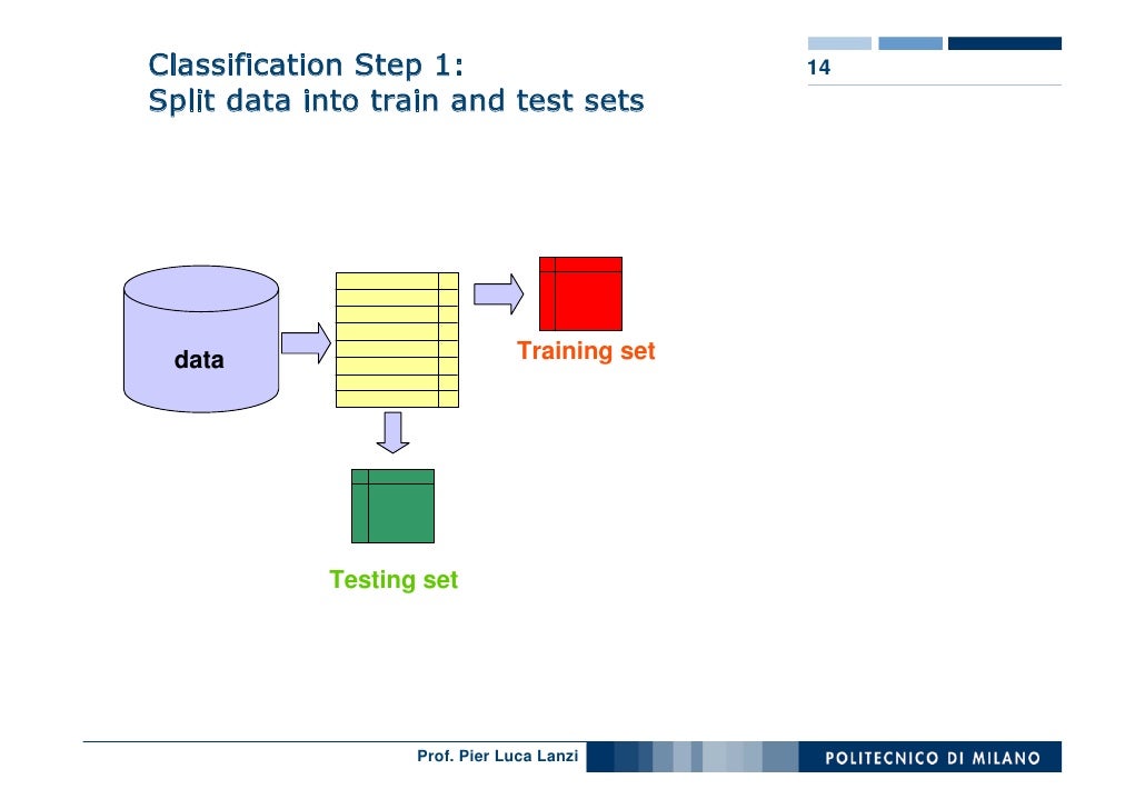
We already have our data loaded into a DataFrame in R, so we'll put 80% of the data into a training set and the remaining 20% of the data into a testing set: 

Since the initial dataset contained 150 plants, our training set contains 120 plants and our testing set contains 30 plants. 

At this point, we're ready to build a neural network to classify these plants. But this post has been a long read and if you're new to the subject, you'll need time to digest everything. So I'll stop the post here and in the next post, we'll continue our descent by assembling a neural network and training it so that it can correctly tell us the species of a flower given only the petal and sepal measurements.