In the previous post, we fiddled with data and set out for an ambitious task of classifying plants. We ended that post after having downloaded, prepared, and partitioned our data, resulting two non-overlapping sets of data: a test set and a training set.
We'll continue now by building, training, and evaluating a neural network to classify these flowers.
First, we'll need to separate the values that we'll use as input to the network from the values we're intending to use as the output from the network. In other words, we need to place all the sepal and petal widths and lengths into a bag that the network can read, and all the species corresponding to the individual sets of sepal and petal widths and lengths into another bag. That way, when the network trains, it only takes into account the 4 inputs. When it produces an output, we can use the other bag (the one with species inside) to see if the network has predicted the species correctly.
Before doing that, we'll need to convert the individual species into an integer representation. This is done because MXNet (the platform we'll use to train neural networks) doesn't really care what the categories actually are. From the perspective of the network, it's just doing mathematical operations and tweaking those operations depending on if we approve of the operations' output.
To make this conversion, we use the following lines of code:

This creates a new column in both training and testing sets that has a value of 1 for Iris setosa, 2 for Iris versicolor, and 3 for Iris virginica.
We then want to separate the inputs (sepal and petal measurements) from the labels (the species). We can do that with the following lines of code:

Perhaps now is a good time to pose a question that vivifies the astounding nature of machine learning: if you were to be given sets of numbers representing flower petal and sepal measurements, along with the species, how long would it take you to empirically (just by looking at the data) develop an intuition to discern the species? For humans, this is undoubtedly a difficult task--it would take any non-savant months to even begin exhibiting any accuracy. We'll soon see whether neural networks consider this task difficult as well.
Now that we've separated input from output, we can construct and train a network. MXNet has two ways for constructing networks: a fine-grained method of construction in which one builds the network layer-by-layer and a high-level alternative in which one simply specifies a small bit of information regarding construction and training. For simplicity, we'll take the latter approach.
The network can be constructed and trained using this snippet of code:
 To anyone that isn't intimate with MXNet, this piece of code is absolute gibberish. So let's see what the network looks like if drawn as a picture:
 The network can be envisioned as a network of three layers: one input layer with 4 nodes (layer 1), one hidden layer with 10 nodes (layer 2), and one output layer with 4 nodes (layer 3). All nodes in layer 1 are connected to all nodes in layer 2; all nodes in layer 2 are connected to all nodes in layer 3.
So what do the nodes actually represent? In the input layer, the nodes represent the values of petal width, petal length, sepal width, and sepal length for a specific flower. In the output layer, the nodes represent the probabilities for each of the 4 species of plants (actually there's three but I made a math mistake and constructed the network such that there are four nodes, but maybe there's some utility in showing that the network is agnostic to however many classes I purportedly have).
What do the nodes in the hidden layer mean, then? Well, some people interpret the values in the hidden layer to be a "transformation" of the values in the previous layer such that it's easier to distinguish the individual classes from each other. This definition is pretty superfiical, so if you want a deeper interpretation and have a solid education in linear algebra, you can probably use a more math-y tutorial to get one.
Okay, so once you've executed that last line of code, MXNet should erupt in training messages. It should end with this note:
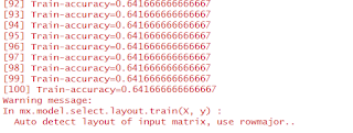 Very spammy and very red. But once it's stopped spamming the console, we can see how well it's trained. To do this, we'll use the cases in our test set that we haven't touched for a while. Remember that we partitioned 20% of our training cases into a testing box for safe keeping until we're done training. Now that we're done training, we can use these cases, which the network has never seen before, to see if it actually learned something useful.
We can get predictions for the cases in the test set with the following lines of code. The predictions are actually probabilities that the case is each species, so to get actual predictions, we need to get the species with the maximum predicted probability:

Okay, so now that we have our predictions, we can compare the predictions to ground-truth labels to see if this network exhibits some accuracy. We can do that with these lines of code:
 What does this mean? This table shows the counts of each class that the network predicted versus the counts of each class that the ground truth shows. We can see that the prediction labels contain 9 values of 1 (species Iris setosa), which is the exact value that the ground truth labels has. That's a good thing. However, the test set says that there are 11 cases of species 2 (Iris versicolor) whereas the network says there are only 10 cases. Oops. We can see that the network misclassified one Iris versicolor as an Iris virginica, as the prediction labels contain 11 cases of value 3, whereas the ground truth labels say that there's only 10.
Okay, so the network messed up on one case out of 30. That's still a lot better than I would do. However, trying to gauge the "quality" of a classifier by seeing how it performs on a testing set and just comparing the max predictions is a pretty rudimentary way of quantifying quality. Let's use a more elegant method.
A more elegant approach to quantifying quality is the AUC (area under curve) score. By "curve", I mean the ROC (receiver operator curve), which is depicted below:
The receiver operator curve is the sensitivity of a classification model (in this case, a neural network) plotted as a function of 100-specificity of the model. In effect, it's the true positive rate (TPR) plotted as a function of the false positive rate (FPR). This is generated by considering the classification that that we're doing, which has 3 individual species/classes (and is therefore multinomial), as 3 separate binary classification (true or false) tasks and altering the predicted probability threshold that we consider a prediction "true" (i.e. anything above probability 0.2 is true, or 0.5, or 0.7). For each threshold setting, we get a TPR and FPR value that we can plot as a point on the ROC. Once we generate an ROC for each binary classification task, we can get the areas under each ROC and average them to get a cumulative AUC score for the multinomial classification task.


We'll continue now by building, training, and evaluating a neural network to classify these flowers.
First, we'll need to separate the values that we'll use as input to the network from the values we're intending to use as the output from the network. In other words, we need to place all the sepal and petal widths and lengths into a bag that the network can read, and all the species corresponding to the individual sets of sepal and petal widths and lengths into another bag. That way, when the network trains, it only takes into account the 4 inputs. When it produces an output, we can use the other bag (the one with species inside) to see if the network has predicted the species correctly.
Before doing that, we'll need to convert the individual species into an integer representation. This is done because MXNet (the platform we'll use to train neural networks) doesn't really care what the categories actually are. From the perspective of the network, it's just doing mathematical operations and tweaking those operations depending on if we approve of the operations' output.
To make this conversion, we use the following lines of code:
This creates a new column in both training and testing sets that has a value of 1 for Iris setosa, 2 for Iris versicolor, and 3 for Iris virginica.
We then want to separate the inputs (sepal and petal measurements) from the labels (the species). We can do that with the following lines of code:
Perhaps now is a good time to pose a question that vivifies the astounding nature of machine learning: if you were to be given sets of numbers representing flower petal and sepal measurements, along with the species, how long would it take you to empirically (just by looking at the data) develop an intuition to discern the species? For humans, this is undoubtedly a difficult task--it would take any non-savant months to even begin exhibiting any accuracy. We'll soon see whether neural networks consider this task difficult as well.
Now that we've separated input from output, we can construct and train a network. MXNet has two ways for constructing networks: a fine-grained method of construction in which one builds the network layer-by-layer and a high-level alternative in which one simply specifies a small bit of information regarding construction and training. For simplicity, we'll take the latter approach.
The network can be constructed and trained using this snippet of code:

So what do the nodes actually represent? In the input layer, the nodes represent the values of petal width, petal length, sepal width, and sepal length for a specific flower. In the output layer, the nodes represent the probabilities for each of the 4 species of plants (actually there's three but I made a math mistake and constructed the network such that there are four nodes, but maybe there's some utility in showing that the network is agnostic to however many classes I purportedly have).
What do the nodes in the hidden layer mean, then? Well, some people interpret the values in the hidden layer to be a "transformation" of the values in the previous layer such that it's easier to distinguish the individual classes from each other. This definition is pretty superfiical, so if you want a deeper interpretation and have a solid education in linear algebra, you can probably use a more math-y tutorial to get one.
Okay, so once you've executed that last line of code, MXNet should erupt in training messages. It should end with this note:
We can get predictions for the cases in the test set with the following lines of code. The predictions are actually probabilities that the case is each species, so to get actual predictions, we need to get the species with the maximum predicted probability:

Okay, so now that we have our predictions, we can compare the predictions to ground-truth labels to see if this network exhibits some accuracy. We can do that with these lines of code:

Okay, so the network messed up on one case out of 30. That's still a lot better than I would do. However, trying to gauge the "quality" of a classifier by seeing how it performs on a testing set and just comparing the max predictions is a pretty rudimentary way of quantifying quality. Let's use a more elegant method.
A more elegant approach to quantifying quality is the AUC (area under curve) score. By "curve", I mean the ROC (receiver operator curve), which is depicted below:
 |
| stolen from https://www.medcalc.org/manual/_help/images/roc_intro3.png |
The AUC for a classfier that is completely random (no knowledge whatsoever) is 0.5 and is shown in the above picture as a dotted line. The AUC for a classifier that is perfect is 1.0. A good heuristic to interpret AUC scores is like school grades, where A is (100-90), B is (89-80), C is (79-70), D is (69- 60) and F is (59-0).
AUC scores are an elegant way of quantifying classifier quality because they take into account more information than just whether the max probability is the correct class. If a classifier gave a case that is supposed to be species 3 an output probability vector of (0.3, 0.3, 0.4), that's of much less quality than a classifier than gives an output probability vector of (0.01, 0.01, 0.98). Ideally, the probabilities of the incorrect classes should be minimized, and the probability of the correct class should be maximized. AUC score captures all that.
Okay, so let's go ahead and calculate the AUC score for our neural network. That can be done with these lines of code (you need to install another package, pROC):
One those lines of code are executed, R shows you the calculated AUC score:

We can see that the AUC score for the network is 0.9848. It's not a perfect classifier (because the AUC score isn't 1.0), and we saw that when we compared the counts of predicted species to the ground truth labels. But nevertheless, 0.9848 is a great AUC score (within the A range).
So there we have it: we've trained a neural network to accurately classify flowers just given their sepal and petal measurements and it took the network less than a second to learn it all. That's much faster than human ability.
So what next? Well, we can either delve into image classification (CNN's), time series classification (RNN's), or tackle more basic classification problems. You'll see what I've decided to continue our descent doing in the next post.
Comments
Post a Comment