Let's continue our descent by evaluating how good our heart disease classifier is.
We can do this by generating predictions on the test set and see how the predictions compare to the test set's ground truth labels. That can be done with the following lines of code:
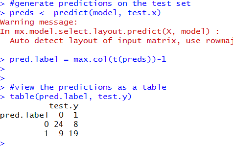 At the bottom we can see that the classifier predicted 24 true negatives, 9 false positives, 8 false negatives, and 19 true positives. That's pretty okay. There is obviously some inaccuracy in the predictions, but let's calculate the accuracy anyways. (24+19)/(24+19+8+9)=71.6.
So the test accuracy was 71.6, while, if you recall from the last post, the training accuracy was nearing 90%. This disparity between training and testing accuracy is a result of overfitting. Essentially, 50,000 training loops was too much training for this little of data. The resulting network overfit to the noise inherent in the training data and, as a result, failed to generalize as well on the test set. Therefore, the testing accuracy can be improved if I were to retrain the network and conduct, say, 30,000 training loops instead.
Let's calculate the AUC score to really evaluate the performance of this model.
 The AUC score for this network is 0.71. That's in the C-range, so we can consider this to be an okay, average-performing network.
Okay, so we have shown that neural nets have some utility as an identifier for heart disease. With some optimization and tweaking, the accuracy can be increased, but this exercise is fruitful in illustrating the power of neural networks.
As for this blog, unfortunately is has to come to an end. I certainly had fun writing it, and I hope that this blog was instrumental in spreading knowledge of neural networks. God speed.
We can do this by generating predictions on the test set and see how the predictions compare to the test set's ground truth labels. That can be done with the following lines of code:
So the test accuracy was 71.6, while, if you recall from the last post, the training accuracy was nearing 90%. This disparity between training and testing accuracy is a result of overfitting. Essentially, 50,000 training loops was too much training for this little of data. The resulting network overfit to the noise inherent in the training data and, as a result, failed to generalize as well on the test set. Therefore, the testing accuracy can be improved if I were to retrain the network and conduct, say, 30,000 training loops instead.
Let's calculate the AUC score to really evaluate the performance of this model.
Okay, so we have shown that neural nets have some utility as an identifier for heart disease. With some optimization and tweaking, the accuracy can be increased, but this exercise is fruitful in illustrating the power of neural networks.
As for this blog, unfortunately is has to come to an end. I certainly had fun writing it, and I hope that this blog was instrumental in spreading knowledge of neural networks. God speed.
Comments
Post a Comment