Partitioning Heart Data

We'll continue our descent by loading, pre-processing, and partitioning the heart disease data. This process will be similar to our previous experiment, but it'll be using the heart disease dataset instead of the iris dataset.

First, we'll load the heart disease data into a dataframe. That can be done with the following lines of code. We'll also rename the columns to be reflective of the dataset's documentation.

The "ca" and "thal" columns have some null values, so let's just remove those rows from the dataframe. There are ways to impute the data rather than just getting rid of the records, but those methods go beyond the scope of this blog and thus we'll pick the easy way out.

Afterwards, we have a couple of categorical variable, if you can recall from the previous post. As they're read in, they're represented by integral values. I'm actually not sure how mxNet deals with these. Either they can be considered categorical values and mxNet implicitly forms a sparse vector of booleans or mxNet might just treat them as true integers, with a false scaling to them. To prevent the latter from happening, I'm going to manually construct the sparse vectors of booleans for each categorical variable. Note that this observation was made while doing a bit of experimentation with this dataset and mxNet. Without splitting these categorical columns into sparse vectors, I simply couldn't get the trained network to converge to a solution that outperformed randomness.

Let's also generate our output boolean. The dataset's output is a categorical value of 0-4, where 0 is a lack of heart disease and anything above 0 represents heart disease of increasing severity. There wasn't too detailed of documentation regarding the delineation of values 1,2,3,4 so I'm going to go ahead and just clump all the positive outputs together as a 1 that indicates the presence of heart disease.

Okay, so after our categorical variables have been expanded, we're going to want to partition a training and testing set. Let's randomly generate indices for both sets and partition the original dataframe into testing and training dataframes. Like last time, we'll use an 80:20 ratio for training and testing set size.

Once we have our training and testing sets, we can partition the ground truth labels from the inputs. Let's do that.

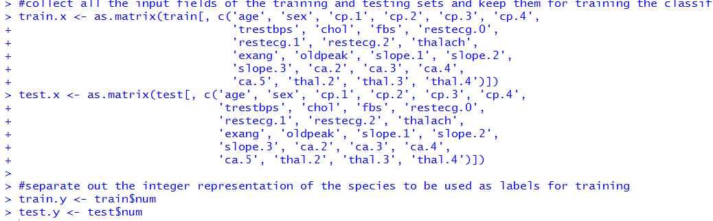Okay, so there we have it. We have both training and testing sets and for each set we have inputs and ground truth labels. In our training and testing sets, categorical variables have been expanded from integral values to vectors of boolean values. Let's hope that this yields a dataset that allows for convergence upon a solution.

Let's continue in the next post by attempting to train this network.