Training a Heart Disease Classifier

As I begin writing this post I realize that we're not training a heart disease predictor, per se, as the classification task at hand isn't really to divine the onset of heart disease in the distant future. Rather, we're really training a heart disease classifier that identifies heart disease given test results, vital measurements, and demographic information. While much less cool than a predictor, this is still a pretty difficult task and I'm certain the definition of "heart disease" might present some aspects of ambiguity and subjectivity between cardiologists. To illustrate the difficulty of this task, you might ask yourself: if you were given the sex, angina status, heart rate measurements, cholesterol measurements, and EKG results of a patient, would you be able to diagnose that patient as having heart disease?

Anyways, let's go ahead and train this network. That can be done with these lines of code. Execution of these lines of code takes about 20 minutes on an i7-6500U.

We can see that there are a bunch of parameters for this model-construction function "mx.mlp" and I'll explain those.  The data and label parameters contain the matrices of inputs and ground truth values of the training set. The hidden node parameter is a vector of integers that specifies how many nodes are in each hidden layer. In this case, we're building a network with two hidden layers of 10 units each. The out_node parameter specifies the number of output nodes: 2, because we're regressing the probability of the presence of heart disease and the presence of a lack of heart disease. The out_activation parameter specifies the activation function for the output. In this case, we're using softmax, which is essentially a multiclass adaptation of the logistic regression function. Finally, we have our number of rounds, our batch size (we're doing full-batch learning), our learning rate, and our momentum.

These parameters have been tweaked while training to converge upon a decent solution.

You might notice that we're using an activation function that might be a little strange. This "softrelu" is like the rectified linear activation function except that it asymptotically approaches zero as the input tends to negative infinity. This is useful because it's smooth and therefore differentiable. Also, ReLU's have this terrible defect that I was experiencing while attempting to train this network where they have a chance at dying completely if they reach a point where all inputs to the ReLU's are less than 0 (weights are negative and inputs are positive). If a ReLU reaches this situation, it effectively can only output 0, as the derivative of the ReLU activation function can only be positive given positive inputs.

Okay, so after the training has been conducted, we can look at the results. The R console should show:

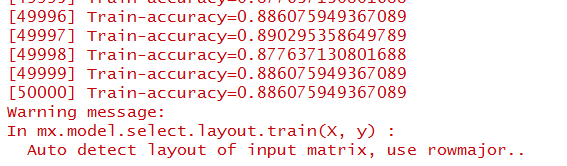Towards the end, we can see that training accuracy was nearing 90%. That's pretty promising. Even though this accuracy is lower than what we saw on the iris dataset, it's important to keep in mind that this is a much more difficult classification task and presents a facade of a very complex physiological system.

Let's continue in the next post to evaluate actually how good this model performs on the test set and we'll also wrap things up.